Using theoretical formulas to optimize costs in practice?
Götz-Andreas Kemmner
At first glance, lot-sizing methods for reducing the overall costs of warehousing and procurement appear very interesting. However, in order to fully exploit the potential, users must also be aware of the limitations of lot-sizing methods and be aware that they cannot take into account all interdependencies throughout the company. The right methodological expertise is therefore required across the entire supply chain to ensure that it is used at the right strategic point.
Hardly any other topic has been and still is the subject of so many dissertations as lot size optimization. This at least shows that the optimization of batch sizes does not yet seem to have been sufficiently solved in theory. The topic is also hotly debated in practice, because for the batch size recipes to work here, you have to understand exactly how they work and where their weak points lie.
Objectives of lot-sizing procedures
The batch size method is intended to calculate an optimum between inventory costs on the one hand and procurement costs for in-house production or external procurement on the other, in order to minimize the total costs in a comparatively small segment of a holistic supply chain. The problem here is that an individual batch size decision, for example in purchasing or for a specific value creation step in production, does not necessarily have to be beneficial for the overall optimum of the supply chain. But that is ultimately the point.
Although it is only about reducing the costs of one good, interdependencies between individual goods must be specified in advance. Only then can the optimum batch size procedure be considered. So never start a batch size project without first taking a look at the entire supply chain. The basis of all batch size calculations is consequently the determination of the relevant costs.
Update 2021 : follow this link for a more up-to-date article
Cost types for lot size optimization
In general, there are two types of costs that react in opposite directions: inventory costs and procurement costs. Warehousing costs are made up of a whole range of cost types. In addition to the interest on the tied-up capital, this also includes other types of costs, which are often significantly higher. These are primarily: costs for aging and wear, loss and breakage, transportation and handling within the warehouse, storage and depreciation as well as warehouse management and insurance.
Procurement costs for in-house or external production primarily include ordering costs, rebates, bonuses, discounts, additional costs for unfavorable order or production quantities, transport, insurance and packaging costs, order processing costs and, of course, setup costs.
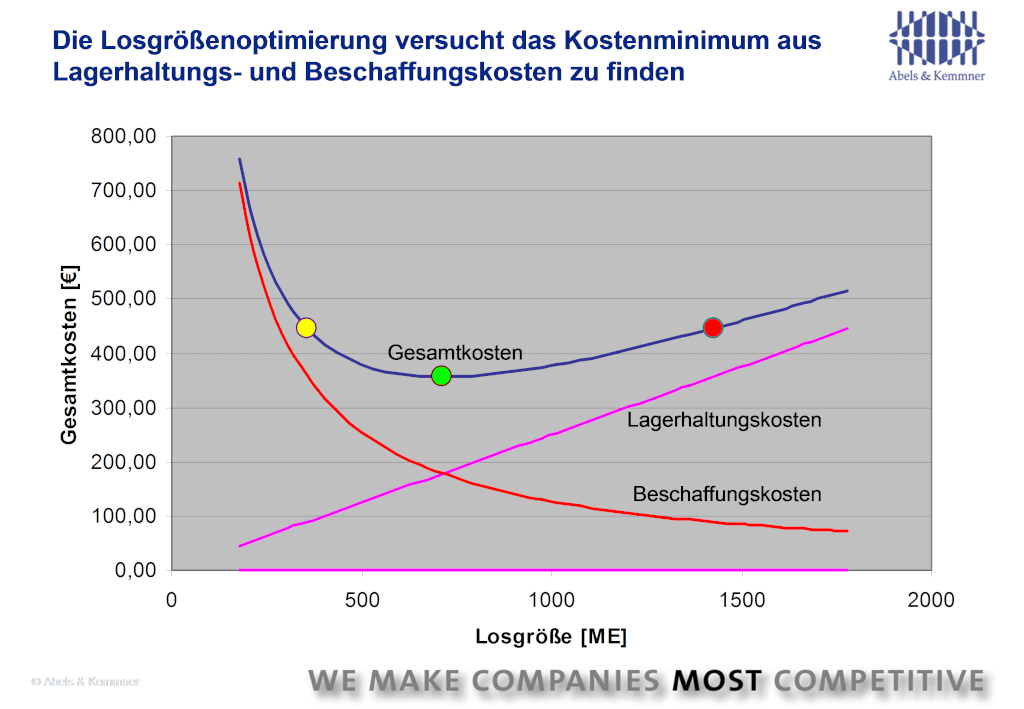
Larger batch sizes in procurement or production lead to higher inventories and therefore higher warehousing costs. These generally increase in proportion to the batch size, while procurement costs fall degressively. A simple example: If the same absolute transportation costs are incurred for one ordered part as for two parts, then if two parts are ordered, each part only bears half of the transportation costs (see Figure 1). In order to bring these different cost curves to an overall optimum, different procedures have been and are being developed, which are summarized under batch size procedures. On the one hand, application requires methodological expertise within this discipline, but it is also important to look at the business as a whole.
The most important lot-sizing methods
With lot-sizing methods, a distinction is usually made between static methods and dynamic methods. Static methods (Andler method) do not consider production or order requirements that vary over time, but only the total quantity required within an observation period and are therefore only approximate calculation methods.
Dynamic methods or periodic lot-sizing methods consider, for example, the varying demand per week over a period of time. They also calculate batch sizes per week and on a rolling basis. They are therefore fundamentally more demand-oriented and can thus adapt to changing requirements. This group of procedures includes
- the Wagner-Whitin method
- the part-period method (piece-period equalization method)
- the unit cost method (sliding economic lot size method)
- the Groff process
- the Silver Meal process.
The large number of different methods can be explained by the fact that no one has yet been able to accurately depict the complex reality in a formula. In this respect, all lot-sizing methods are only approximate solutions. However, some are closer to the optimum than others. The procedures listed above must therefore be understood very precisely in order to be able to use them effectively.
All of the above methods describe the interaction or counteraction of inventory costs and procurement costs in a single-stage, single-product production process without capacity limits. An example: You have a printing machine on which you have mounted a printing plate. Setting up the press will cost you paper and ink regardless of your manpower, as you will be producing waste for quite some time until you have set up the press correctly. As you have to produce the same document over and over again, the only dilemma you face is that of high production batches and therefore low pro rata set-up costs on the one hand and high stock levels and inventory costs on the other. The batch size calculation formulas of the classic methods attempt to describe a “trade-off” formula for precisely this situation.
However, the question of a batch size only really arises when more than one product is manufactured. Even if several products are manufactured on one system, our formulas are correct, as long as the batch sizes of the two products do not influence each other due to limited machine capacity. However, this is often the case.
Purchasing must also optimize at a higher level
The situation is similar in procurement. Here, too, it is often not possible to make an isolated batch size analysis for a single product. On the one hand, several different products can “share” procurement costs: think, for example, of a truck that can be loaded with several products. On the other hand, it is often a matter of getting the truck full in order to achieve the lowest possible transport costs. Several products are therefore ordered together and thus influence each other with regard to their order quantities. With the supposedly “optimal” order quantity for one product, I automatically limit the scope of order quantities for the other products.
Let’s take another look at production: In a production process in which I optimize batch sizes from one production stage to the next, I work with 450 pieces in a production order for turning. For the subsequent milling, I have determined 380 pieces as “optimal” and for the subsequent electroplating I arrive at a batch size of 1250 pieces. The result: intermediate stocks that were not taken into account in the individual case calculation and possibly several “optimum” production quantities that have to be produced directly one after the other. As you can see, as simple as a formula is in individual cases, the reality is complex.
More complex is more precise, but also more difficult
There are batch size optimization methods that take the entire process chain into account. However, if we now also realistically take into account that capacities at the individual production stages are limited, reality can no longer be fully calculated with all the given interdependencies and limitations.
Let’s take another brief look at some of the formulas using a brief historical outline in order to evaluate them in concrete terms.
Andler is often too simple
In 1929, Kurt Andler developed a formula for calculating an economic batch size. The Andler formula determines the minimum of the total cost curve in Figure 1. When calculating the lot size, Andler assumed that the total quantity required of an item in a planning period, e.g. one year, is known. The formula now derives the batch size that should always be used for ordering from inventory costs on the one hand and procurement costs on the other. As the lot size remains constant over the planning period, this is also referred to as a static lot size formula.
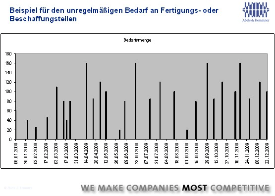
In practice, however, production or order requirements are not constant over a planning period, typically less than one year. Rather, they follow each other irregularly and are of different heights (Fig. 2).
Consequently, in these cases there must be a more precise solution for an economical batch size. Two Americans provided the decisive answer back in 1958.
Wagner-Within is very precise
Mr. Wagner and Mr. Whitin developed a batch size calculation method with which dynamic batch sizes could be calculated. This mathematical solution takes into account the fact that the decision on a first batch size in the period under consideration automatically limits the scope for the design of subsequent batch sizes. The Wagner-Whitin method determines a sequence of lots with different sizes and different time intervals, which minimizes the total costs. The result is a scientifically precise answer to the question of the correct batch sizes for single-stage, single-product production without capacity limits. The Wagner-Whitin method can even be calculated by hand, but becomes very complex for batch sizes for countless products, even for calculating machines of the time. Approximation methods with simpler calculation methods were therefore needed, which computers could cope with at the expense of accuracy. For example, the Part Period method was developed in 1968, the Silver-Meal method named after its developers in 1969 and the Groff method in 1979.
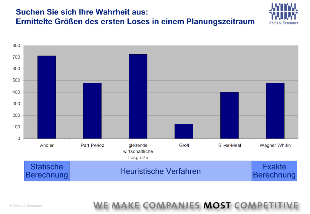
As these approximation methods make various simplifications, they also determine the optimum costs for different batch sizes. The deviations from the precisely calculated Wagner-Whitin method can be very significant, as Figure 3 shows. The heuristic methods for batch size optimization are sometimes far removed from the exact results of the Wagner-Whitin method, as the example of a demand time series shows.
In the mid-1990s, computers were fast enough to be able to apply the Wagner-Whitin method to a large number of articles. However, it is still missing in most of today’s standard ERP systems. The systems still offer the Andler formula, which is justified for certain aspects, and heuristic procedures. Users are satisfied with this, partly because they don’t know that there are better methods and partly because they have become accustomed to all these methods over the years. The Wagner-Whitin process is currently not usually found in ERP systems. However, there are add-on systems for supply chain optimization that Wagner-Whitin offers. You should therefore take a look at them. If you are ready to search for your optimum batch sizes with Wagner-Whitin, here are a few final tips:
Avoid incorrect imputed costs
When considering costs, an imputed value is usually used for both storage costs and procurement costs. This is helpful for approximate calculations, but not sufficient for a more differentiated view. Let’s first take a look at this using the example of procurement costs:
You may be familiar with the case of the eraser that costs EUR 50 to buy, a case that was in the press a few years ago when people were discussing the advantages of buying over the Internet. How do you arrive at such a value for a cent item in a calculation? Quite simply, you not only look at the purchase price of the item, but also take into account the costs incurred in procuring the eraser. Someone may write a requirement, which may be signed off by the line manager and then forwarded to the purchasing department. The purchasing department may not request three quotations for the eraser, but rather the purchaser orders the desired eraser via SAP from an already negotiated framework agreement. To do this, he must create and release a purchase order. The order is then printed out, signed and faxed. The original order is filed in a folder.
It becomes clear that “procurement costs” arise here, which can be very high regardless of the price of the goods procured. In our example company, personnel costs of EUR 250,000 are incurred for purchasing in the company. The cost share for the IT software and hardware may amount to a further EUR 15,000. The remaining costs amount to a further EUR 35,000. In total, purchasing and its processes “cost” EUR 300,000 per year. The cost of incoming goods amounts to a further EUR 300,000. In total, ordering and receiving goods costs our company EUR 600,000. There are 11,000 orders a year. This results in an amount of EUR 54.55 per order. The calculation is that simple – and that’s how wrong it is!
What if, instead of 11,000 orders per year, 15,000 orders were placed because orders are placed in smaller batches? With 240 working days in purchasing per year, this would trigger around 62 orders per day instead of just under 46. The costs per order would then be EUR 40. The marginal costs, i.e. the additional costs for each further order, would be 0 euros. With batch size optimization, only the variable order costs that are incurred with each new order are of interest. The fixed cost components only become relevant when they increase due to the increased number of procurement processes.
This marginal cost effect can even occur with cost items that are supposedly incurred with every delivery. Let’s assume that each delivery costs freight costs of 5. if the eraser were the only order placed with the supplier today, then the 5 would be added to the procurement costs of the eraser. But presumably a whole lot of office supplies are delivered every day. The freight costs of the eraser are therefore only a fraction of the 5. Whether one part more or less is supplied by the office materials supplier today is not reflected in the freight costs. The marginal costs are therefore zero.
What remains at the end
The closer you look, the more inaccuracies you find in practice when calculating batch sizes. Nevertheless, batch size calculation is justified. However, you have to understand the individual procedures, applicable boundary conditions and simplifications very precisely. Batch size optimization is therefore not simple supply chain optimization using formulas that can simply be calculated on a PC, but an optimization approach for specialists. They put the application of the method in the right context and adjust the cost calculations so that they are accurate. Anything else is just poking around in the fog.
Keywords: lot size optimization, supply chain, cost reduction, warehousing, procurement
Literature
[1] Harris, F.W.: How Many Parts to Make at Once Factory: The Magazine of Management 10(2):135-136,152 (1913)